Pretreatment chemistry in desalination lives or dies by dose control. Plants are pairing charge-based sensors with old-school jar tests to hold coagulants in the sweet spot, cutting 10–30% or more off chemical use while stabilizing turbidity.
In desalination pretreatment, coagulation/flocculation (C/F) is the first solid–liquid separation stage. The job: destabilize colloids so they clump and settle before hitting sensitive reverse osmosis (RO) trains. Typical inorganic coagulant doses are on the order of 5–30 mg/L (much higher than polymeric aids) (mdpi.com). Feedwater pH must also be managed because ferric coagulants consume more alkalinity, often requiring acid addition (mdpi.com).
The stakes are clear: overdosing wastes money and makes sludge; underdosing leaves turbidity and organics that foul RO. At Fujairah II SWRO (a hybrid plant cited as the world’s largest), operators dose ferric chloride for pre‑sedimentation and carefully adjust pH to prevent scaling (mdpi.com). Downstream, that protects brine-stressed membranes—whether full-scale SWRO systems or pretreatment-driven trains feeding ultrafiltration (UF) ahead of RO.
Charge-based monitoring and control
Modern pretreatment is leaning on automatic sensors to adjust dosing in real time as raw-water turbidity and organics swing. A core device is the streaming current monitor (SCM), which measures the net electrokinetic charge of coagulated water. When positively charged coagulant exactly neutralizes the raw-water colloidal charge, the streaming current reading goes to near 0.0 (WaterWorld).
In practice an SCM uses a membrane zeta‑potential sensor to detect net charge; a “0.0” reading indicates optimal dose under good mixing (WaterWorld). Negative or positive streaming current shows under‑ or over‑dosing, so operators trim the feed—often via an accurate dosing pump—to hold near setpoint. Philadelphia’s Baxter WTP trialed SCM on parallel trains (charge‑neutralization vs sweep flocculation) and found it effective for stabilizing dose in real time (WaterWorld). As raw natural organic matter rises, the SCM signal drops, flagging the need for more coagulant (WaterWorld).
There are caveats: SCM accuracy depends on stable pH and is most reliable below pH ~7 for aluminum coagulants and ~6 for iron; above those levels signals become sluggish and may mislead—one review noted poor control when pH ≥7 (mdpi.com) (mdpi.com). Regular calibration and settle‑point checks—often by jar test—are required (mdpi.com) (mdpi.com). When properly deployed, SCM‑based control has delivered significant coagulant savings; Zhang and Luo describe large savings using a neural‑network model with streaming‑current feedback (mdpi.com).
Particle counters for fine‑scale visibility
Turbidity meters can miss small particulate breakthroughs. Online particle counters fill that gap by counting and sizing individual particles with a laser sensor, delivering counts in bins (e.g., >1 µm, >5 µm) (Micron Scientific). One scheme routes a post‑flocculation side‑stream through a tube settler (to remove larger flocs) and then into a counter; the resulting “primary particle” concentration reflects residual colloids (AguaClara).
Any uptick in fines signals under‑dosing; a drop (or zero count) suggests possible overdosing. Modern counters such as the PAMAS WaterViewer measure continuously and flag issues more reliably than turbidity alone (Micron Scientific). This is especially valuable ahead of a gravity clarifier or media filtration like a sand/silica filter, where fine floc carryover can otherwise sneak through.
Zeta‑potential and pH feedback loops
Zeta potential (particle surface charge in suspension) is a conceptual cousin to streaming current. On‑line zeta‑meters (e.g., Malvern Zetasizer WT) use micro‑electrophoresis or acoustic methods to track charge and hold dose to a target range. Inline pH probes ensure coagulants are applied in their optimal pH window; ferric flocs form best at pH ~5–6, alum at ~6–7. Plants often run a dual‑loop: SCM or zeta to control coagulant dose and pH to maintain neutralization setpoints—pragmatic when feeding alum via an automated coagulant skid (mdpi.com).
Other online signals—including feed turbidity, UV254 (organic absorbance), and conductivity—are increasingly pushed into SCADA or AI controllers. A 4‑year Moroccan plant study found data‑driven models, once trained, provided robust real‑time setpoints for dosing and integrated into operator advisory systems (mdpi.com). The trend is toward “feed‑backward” control: measure post‑coagulation quality (charge, particles) and adjust pump rates accordingly, rather than conservative overfeed to avoid upsets.
Measured savings and stability gains
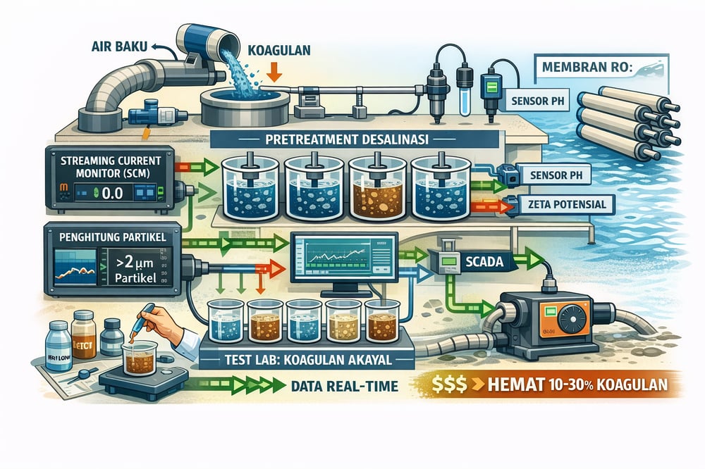
Plants report that these tools can cut dosing by 10–30% or more compared to fixed feed rates; one full‑scale trial reported “significant savings” with automated charge‑based control versus manual practice (mdpi.com). Beyond savings, real‑time control avoids swings in turbidity. Upsets can be corrected within minutes rather than hours, shielding downstream media and membranes. Plants without such control often resort to conservative overdosing to avoid MLE events; with online monitors, dose holds closer to the true optimum.
In one case study, a site with 110 NTU raw turbidity consistently achieved <10 NTU after coagulation by using a feedback controller on streaming current and pH (mdpi.com). ANN‑based controllers trained on jar‑test data delivered significant chemical savings in Canadian and Chinese waterworks (mdpi.com). Even a 10% saving in coagulant can translate to tens of thousands of dollars per year in large plants. Consistent effluent turbidity helps meet stringent drinking‑water standards of ~0.5 NTU (id.scribd.com) and reduces RO fouling events—each avoided clean cuts downtime for RO, NF, and UF systems.
Jar testing to set chemistry
Despite the rise of sensors, the bench‑top jar test remains the authoritative way to choose and calibrate chemicals before commissioning or after a major source‑water shift. A jar test simulates rapid mix, flocculation, and settling across multiple jars to compare doses and types of coagulant and polymer (OApen) (OApen).
The playbook:
1) Sample collection: pull a representative raw feed (seawater or brackish) and record turbidity, pH, temperature, salinity. 2) pH adjustment if needed: dedicate jars at different pH using HCl or NaOH to test optima (alum often near pH 6.5–7.5). 3) Stock solutions: prepare known concentrations (e.g., 1 g/L ferric chloride or alum) and dose to targets such as 5, 10, 15, 20 mg/L (Sugar Process Tech). 4) Rapid mix: 100–150 rpm (G ≈ 200–600 s⁻¹) for ~1–2 minutes. 5) Slow flocculation: 30–40 rpm (G ≈ 30–70 s⁻¹) for ~10–20 minutes; add polymeric flocculants at the start of this stage. 6) Settling: 15–30 minutes, representing gravity clarification. 7) Measurement: sample ~2″ below the surface; measure turbidity (NTU), residual coagulant, suspended solids; note floc size and firmness. 8) Evaluation: pick the lowest turbidity with good, settleable flocs; if higher doses cause restabilization or very fine flocs and worse turbidity, that marks the overdose point (OApen) (OApen).
Costing matters. If Jar A (ferric chloride at 10 mg/L) reduces turbidity to 5 NTU and Jar B (polymer at 0.5 mg/L) gives 3 NTU, compare costs: at $0.5/kg for ferric chloride and $1.50/kg for polymer, 10 mg/L FeCl₃ costs $0.005/m³ while 0.5 mg/L polymer is $0.00075/m³—far cheaper and clearer. Screening across cationic vs anionic, high‑ vs low‑charge polymers and alternative coagulants (alum vs PAC vs polyaluminum chloride) often reveals performance differences. Factorial jar designs let teams vary coagulant dose and flocculant dose, or coagulant type, or include turbidity‑versus‑pH interactions; for complex feeds like seawater with algae, some plants include algal toxins or organic surrogates in jars (OApen) (OApen).
Real outcomes are specific: a source water might run best at pH 6.5 with 15 mg/L ferric chloride plus 0.5 mg/L cationic polymer. Jar tests should be repeated when seasons change—think algae blooms or heavy runoff—and they calibrate the real‑time control setpoints. The operating target for a streaming‑current or zeta loop is commonly the reading that corresponded to “good coagulation” in the jars. Selected chemicals then slot into dosing systems and storage, from liquid flocculants to polyaluminum coagulants, supporting pre‑filters like cartridge filters before UF pretreatment or RO.
Integrating sensors with treatment trains
In practice, a best‑practice pretreatment system integrates periodic jar testing to anchor the chemistry with continuous online sensing (SCM, particle counts, zeta‑potential, pH) to follow it in real time. That dual approach keeps effluent turbidity and SDI (silt density index, a fouling proxy) steady while trimming OPEX through leaner chemical usage. The goal is consistent feed to filters and membranes—whether a gravity stage ahead of a clarifier or multi‑media sand beds feeding a UF skid protecting downstream RO.
For many desal plants, that also means standardizing on high‑quality coagulants and flocculants, pairing them with accurate chemical dosing, and verifying performance with counters. On troublesome days, a laser counter will see what a turbidimeter can miss; on calm days, a near‑zero SCM reading is a green light to keep feeding lean.
Sources and further reading
Guidelines and dose ranges come from Jaber et al. (2023) (mdpi.com) (mdpi.com). Streaming‑current feedback and online monitors are documented by Kramer & Horger (2001) and Johnson & Pernitsky (2011) (WaterWorld) (WaterWorld). The open textbook “Jar Tests for Water Treatment Optimization – How to Perform Jar Tests: a Handbook” (Pivokonský et al., 2017) details bench methods (OApen) (OApen). Additional context on coagulant automation and particle counting methods appears via AguaClara (aguaclara.github.io) and Micron/PAMAS (micronscientific.co.za). A cited drinking‑water turbidity limit reference is available via id.scribd.com.
